This is a post about complex specified information (CSI). But first, I’d like to begin with a true story, going back to the mid-1960s. A Cambridge astronomer named Anthony Hewish had designed a large radio telescope, covering more than four acres, in order to pick out a special group of objects in the sky: compact, scintillating radio sources called quasars, which are now known to be the very active and energetic cores of distant galaxies. Professor Hewish and his students were finally able to start operating their telescope by July 1967, although it was not completely finished until later on. At the time, Hewish had a Ph.D. student named Jocelyn Bell. Bell had sole responsibility for operating the telescope and analyzing the data, under Hewish’s supervision.
Six or eight weeks after starting the survey, Jocelyn Bell noticed that a bit of “scruff” was occasionally appearing in the data records. However, it wasn’t one of the scintillating sources that Professor Hewish was searching for. Further observations revealed that it was a series of pulses, spaced 1.3373 seconds apart. The pulses could not be man-made, as they kept to sidereal time (the time-keeping system used by astronomers to track stars in the night sky). Subsequent measurements of the dispersion of the pulse signal established that the source was well outside the solar system but inside the galaxy. Yet at that time, a pulse rate of 1.3373 seconds seemed far too fast for a star, and on top of that, the signal was uncannily regular. Bell and her Ph.D supervisor were forced to consider the possibility of extraterrestrial life. As Bell put it in her recollections of the event (after-dinner speech, published in Annals of the New York Academy of Sciences, vol. 302, pp. 685-689, 1977):
We did not really believe that we had picked up signals from another civilization, but obviously the idea had crossed our minds and we had no proof that it was an entirely natural radio emission.
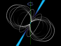
The observation was half-humorously designated Little green men 1 until a famous astronomer, Thomas Gold, identified these signals as rapidly rotating neutron stars with strong magnetic fields, in 1968. The existence of these stars had been postulated as far back as 1934, by Walter Baade and Fritz Zwicky, but no-one had yet confirmed their existence when Bell made her observations in 1967, and only a few astronomers knew much about them.
Here’s a question for readers: was Bell wrong to consider the possibility that the signals might be from aliens? Here’s another one: if you were searching for an extra-terrestrial intelligence, what criteria would you use to decide whether a signal came from aliens? As we’ll see, SETI’s criterion for identifying alien signals makes use of one form of complex specified information. The criterion – narrow band-width – looks very simple, but it involves picking out a sequence of events which is highly surprising, and therefore very complex.
My previous post, entitled Why there’s no such thing as a CSI Scanner, or: Reasonable and Unreasonable Demands Relating to Complex Specified Information, dealt with complex specified information (CSI), as defined in Professor William Dembski’s paper, Specification: The Pattern that Signifies Intelligence. It was intended to answer some common criticisms of complex specified information, and also to explain why CSI, although defined in a mathematically rigorous manner, is not a physically computable quantity. Briefly, the reason is that Professor Dembski’s formula for CSI contains not only the physically computable term P(T|H), but also the semiotic term Phi_s(T). Specifically, Dembski defines the specified complexity Chi of a pattern T given chance hypothesis H, minus the tilde and context sensitivity, as:
Chi=-log2[10^120.Phi_s(T).P(T|H)],
where Chi is the specified complexity (or CSI) of a system,
Phi_s(T) is the number of patterns whose semiotic description by speaker S is at least as simple as S’s semiotic description of T,
P(T|H) is the probability of a pattern T with respect to the most plausible chance hypothesis H, and
10^120 is the maximal number of bit operations that the known, observable universe could have performed throughout its entire multi-billion year history, as calculated by theoretical computer scientist Seth Lloyd (“Computational Capacity of the Universe,” Physical Review Letters 88(23) (2002): 7901–4).
Some of the more thoughtful skeptics who regularly post comments on Uncommon Descent were not happy with this formula, so I’ve come up with a simpler one – call it CSI-lite, if you will – which I hope will be more to their liking. This post is therefore intended for people who are still puzzled about, or skeptical of, the concept of complex specified information.
The CSI-lite calculation I’m proposing here doesn’t require any semiotic descriptions, and it’s based on purely physical and quantifiable parameters which are found in natural systems. That should please ID critics. These physical parameters should have known probability distributions. A probability distribution is associated with each and every quantifiable physical parameter that can be used to describe each and every kind of natural system – be it a mica crystal, a piece of granite containing that crystal, a bucket of water, a bacterial flagellum, a flower, or a solar system. Towards the end of my post, I shall also outline a proposal for obtaining as-yet-unknown probability distributions for quantifiable parameters that are found in natural systems. But although CSI-lite, as I have defined it, is a physically computable quantity, the ascription of some physical feature of a system to intelligent agency is not. Two conditions need to be met before some feature of a system can be unambiguously ascribed to an intelligent agent: first, the physical parameter being measured has to have a value corresponding to a probability of 10^(-150) or less, and second, the system itself should also be capable of being described very briefly (low Kolmogorov complexity), in a way that either explicitly mentions or implicitly entails the surprisingly improbable value (or range of values) of the physical parameter being measured.
There are two things I’d like to say at the outset. First, I’m not going to discuss functional complex specified information (FCSI) in this post. Readers looking for a rigorous definition of that term will find it in the article, Measuring the functional sequence complexity of proteins by Durston, Chiu, Abel and Trevors (Theoretical Biology and Medical Modelling 2007, 4:47, doi:10.1186/1742-4682-4-47). This post is purely about CSI, and it can be applied to systems which lack any kind of functionality. Second, I should warn readers that I’m not a mathematician. I would therefore invite readers with a strong mathematical background to refine any proposals I put forward, as they see fit. And if there are any mathematical errors in this post, I take full responsibility for them.
Let us now return to the topic of how to measure complex specified information (CSI).
What the CSI skeptics didn’t like
One critic of Professor Dembski’s metric for CSI (Mathgrrl) expressed dissatisfaction with the inclusion of a semiotic term in the definition of complex specified information. She wrote:
[U]nless a metric is clearly and unambiguously defined, with clarifying examples, such that it can be objectively calculated by anyone so inclined, it cannot be used as the basis for claims such as those being made by some ID proponents.
She then quoted an aphorism by the science fiction writer Robert Heinlein: “If it can’t be expressed in figures, it is not science; it is opinion.”
From a purely mathematical standpoint, the key problem with the term Phi_s(T) is that descriptive simplicity is language-dependent; hence the number of patterns whose semiotic description by speaker S is at least as simple as S’s semiotic description of T will depend on the language which S is using. To be sure, mathematics can be considered a universal language which is shareable across all cultures, but even if all mathematicians could agree on a list of basic mathematical operations, there would still remain the problem of how to define a list of basic predicates. For instance, is “is-a-motor” a basic predicate when describing the bacterial flagellum, or does “motor” need to be further defined? And does “basic” mean “ontologically basic” or “epistemically basic”?
Another critic (Markf) faulted Professor Dembski’s use of a multiplier in the calculation of CSI, pointing out that if there are n independent events (e.g. 10^120 events in the history of the observable universe) and the probability of a single event having outcome x (e.g. a bacterial flagellum) is p, then the probability of at least one event having outcome x (i.e. at least one bacterial flagellum arising in the history of the cosmos) is not np, but (1–(1-p)^n). In reply, I argued that the binomial expansion of (1–(1-p)^n) can be very closely approximated by (1-(1-np)) or np, when the probability p is very small, as it is for the formation of a bacterial flagellum as a result of mindless, unintelligent processes. However, Markf responded by observing that Dembski introduces a multiplier into his formula on page 18 of his article as a general way of calculating specificity, before it is even known whether p is large or small.
The criticisms voiced by Mathgrrl and Markf are not without merit. Today’s post is intended to address their concerns. The concept I am putting forward here, which I’ve christened “CSI-lite”, is not as full-bodied as the concept employed in Dembski’s 2005 paper on specification. Nevertheless, it is a physically computable quantity, and I have endeavored to make the underlying mathematics as rigorous as could be desired.
The modifications to CSI that I’m proposing here can be summarized under three headings.
Modification 1: Replace the semiotic factor Phi_s(T) with the constant 10^30
First, my definition of CSI-lite removes Phi_s(T) from the actual formula and replaces it with a constant figure of 10^30. The requirement for low descriptive complexity still remains, but as an extra condition that must be satisfied before a system can be described as a specification. So Professor Dembski’s formula now becomes:
CSI-lite=-log2[10^120.10^30.P(T|H)]=-log2[10^150.P(T|H)]. (I shall further refine this formula in Modification 2 below.)
Readers of The Design Inference: Eliminating Chance through Small Probabilities and No Free Lunch: Why Specified Complexity Cannot Be Purchased without Intelligence will recognize the 10^150 figure, as 10^(-150) represents the universal probability bound which Professor Dembski argued was impervious to any probabilistic resources that might be brought to bear against it. Indeed, in Addendum 1 to his 2005 paper, Specification: The Pattern that Signifies Intelligence, Dembski wrote: “as a rule of thumb, 10^(-120) /10^30 = 10^(-150) can still be taken as a reasonable (static) universal probability bound.”
Why have I removed Phi_s(T)? First, Phi_s(T) is not a physical quantity as such, but a semiotic one. Replacing it with the constant figure of 10^30 makes CSI-lite physically computable, once P(T|H) is known. Second, Phi_s(T) is relatively insignificant in the calculation of CSI, anyway, as the exponent of 10 in Phi_s(T) is dwarfed in magnitude by the exponents of the other terms in the CSI formula. For instance, in my computation of the CSI of the bacterial flagellum, Phi_s(T) was only 10^20, which is much smaller than 10^120 (the maximum number of events in the history of the observable universe), while P(T|H) was tentatively calculated as being somewhere between 10^(-780) and 10^(-1170). The exponents of both these figures are very large in terms of their absolute magnitudes: even 780 is much larger than 20, the exponent of Phi_s(T). Thus Phi_s(T) will not usually make a big difference to CSI calculations, except in “borderline” cases where P(T|H) is somewhere between 10^(-120) and 10^(-150). Third, the overall effect of including Phi_s(T) in Professor Dembski’s formulas for a pattern T’s specificity, sigma, and its complex specified information, Chi, is to reduce both of them by a certain number of bits. For the bacterial flagellum, Phi_s(T) is 10^20, which is approximately 2^66, so sigma and Chi are both reduced by 66 bits. My formula makes that 100 bits (as 10^30 is approximately 2^100), so my CSI-lite computation represents a very conservative figure indeed.
Readers should note that although I have removed Dembski’s specification factor Phi_s(T) from my formula for CSI-lite, I have retained it as an additional requirement: in order for a system to be described as a specification, it is not enough for CSI-lite to exceed 1; the system itself must also be capable of being described briefly (low Kolmogorov complexity) in some common language, in a way that either explicitly mentions pattern T, or entails the occurrence of pattern T. (The “common language” requirement is intended to exclude the use of artificial predicates like grue.)
Modification 2: Instead of multiplying the “chance” probability p of observing a pattern T here and now by the number of trials n, use the formula (1–(1-p)^n)
My second modification of Professor Dembski’s formula relates to Markf’s argument that if we wish to calculate the probability of the pattern T’s occurring at least once in the history of the universe, then the probability p of pattern T occurring at a particular time and place as a result of some unintelligent (so-called “chance”) process should not be multiplied by the total number of trials n during the entire history of the universe. Instead one should use the formula (1–(1-p)^n), where in this case p is P(T|H) and n=10^120. Of course, my CSI-lite formula uses Dembski’s original conservative figure of 10^150, so my corrected formula for CSI-lite now reads as follows:
CSI-lite=-log2(1-(1-P(T|H))^(10^150)).
If P(T|H) is very low, then this formula will be very closely approximated by the formula: CSI-lite=-log2[10^150.P(T|H)]. Actually, I would strongly advise readers to use this approximation when calculating CSI-lite online, because calculating it will at least yield meaningful answers, whereas the correct formula does not, owing to the current limitations of online calculators. For instance, if P(T|H) equals 10^(-780), which was the naive upper bound I used in my last post for the probability of a bacterial flagellum arising as a result of a “blind” (i.e. non-foresighted) process, then it is easy to calculate online that since (10^150).P(T|H) equals 10^(-630), and log2(10) is 3.321928094887362, and log2(10^(- 630))=-2092.8147, the minimum value of the CSI-lite for a bacterial flagellum should be approximately 2093, which is well in excess of the cutoff threshold of 1. But if you try to calculate (1-(1-(10^(-780)))^(10^150)) online, all you will get is a big fat zero, which isn’t much help.
Modification 3: Broaden the scope of CSI to include supposedly “simple” cases – e.g. a highly singular observed value for a physical parameter
The third and final modification I’ve made to Professor Dembski’s definition of CSI is that I’ve attempted to broaden its scope. Professor Dembski’s formula was powerful enough to be applied to any highly specific pattern T, be it a complex structure (e.g. a bacterial flagellum) or a specified sequence of digits (e.g. a code). However, Mathgrrl pointed out that SETI doesn’t look for complex signals when searching for life in outer space: instead they look for signals whose range of frequencies falls within a very narrow band. I also started thinking about Arthur C. Clarke’s example of the monolith on the moon in his best-selling novel 2001, and I suddenly realized that the definition of CSI could easily be generalized to cover these cases. In a nutshell: the “surprise factor” attaching to some physical parameter of a system can be used to represent its CSI. This was a very belated recognition on my part, which should have been obvious to me much earlier on. As far back as 1948, the mathematician Claude Shannon pointed out that we can define the amount of information provided by an event A having probability p(A), by the formula: I(A)=-log2(p(A)), where the information is measured in units of bits/symbol (A Mathematical Theory of Communication, Bell System Technical Journal, Vol. 27, pp. 379–423, 623–656, 1948). Subsequently, engineers such as Myron Tribus (Thermostatistics and Thermodynamics, D. van Nostrand Company, Inc., Princeton NJ, 1961) linked the notion of surprise with improbability. Myron Tribus coined the term “surprisal” to describe the unpredictability of a single digit or letter in a word, and hence how surprising it is – the idea being that a highly improbable outcome is very surprising, and hence more informative. More recently, many other Intelligent Design theorists, including Professor Dembski, have already linked complex specified information (CSI) to the improbability of a system, as the presence of P(T|H) in the formula shows. And in 2002, Professor Paul Davies publicly praised Dembski for linking the notion of “surprise” to that of “design”:
“…I think that Dembski has done a good job in providing a way of mathematizing design. That is really what we need because otherwise, if we are just talking about subjective impressions, we can argue till the cows come home. It has got to be possible, or it should be, to quantify the degree of “surprise” that one would bring to bear if something turned out to be the result of pure chance. I think that that is a very useful step.” (Interview with Karl Giberson, 14 February 2002, in “Christianity Today.” Emphasis mine – VJT.)
All I’m doing in this post is explicitly linking CSI-lite to the notion of surprise. What I’m proposing is that the “surprise factor” attaching to some physical parameter of a system (or its probability distribution) can be used to represent its CSI-lite.
I would now like to explain how my definition of CSI-lite can be applied to supposedly “simple” but nevertheless surprising cases – a highly singular observed value for a single physical parameter, an extremely narrow range of values for one or more physical parameters, and an anomalous locally observed probability distribution for a physical parameter – in addition to the complex patterns already discussed by Professor Dembski.
My explanation makes use of the notion of a probability distribution. Readers who may have forgotten what a probability distribution is, might like to think of a curve showing the height distribution for American men, which roughly follows a Bell curve, or what’s known as a normal distribution, in mathematical circles. Many other probability distributions are possible too, of course. If the variable being measured is continuous (like height), then the probability distribution is called a probability density function. (The terms probability distribution function and probability function are also sometimes used.) A probability density function for a continuous variable is always associated with a curve. Most people, when they think of a probability distribution function, imagine a symmetrical curve such as a Bell curve, but for other functions, the curve may be asymmetrical – for instance, it may be skewed to one side. For discrete variables (e.g. the numbers that come up when a die is rolled), mathematicians use the term probability mass function, instead of the term “probability density function.” Here is what the probability mass function looks like for a fair die. With a probability mass function, there is no curve, but there is a set of probabilities (e.g. 1/6 for each face on a fair die), which add up to 1. Even though the probability mass function for a discrete variable has no curve, we can still refer to this function as a probability distribution.
In the discussion that follows, readers might like to keep the image of a Bell curve in their minds, for simplicity’s sake. Readers who are curious can find out more about various kinds of probability distributions here if they wish. In the exposition that follows, the physical parameter being measured may be either discrete or continuous. However, I make no assumptions about the shape of the probability distribution for the parameter in question. One notion I do make use of, however, is that of salience. I assume that it is meaningful to speak of a probability distribution as having one or more salient points. A salient point would include the following: an extreme or end-point (e.g. a uniform probability distribution function over the interval [0,1] has two salient points, at x=0 and x=1), an isolated point (e.g. the probability distribution for a die has six salient points – the values 1 to 6), a point of discontinuity or sudden “jump” on a probability distribution curve, and a maximum (e.g. the peak in a Bell curve). The foregoing list is not intended to be an exhaustive one.
Definitions of CSI-lite for a physical parameter, a probability distribution, a sequence and a structure
CASE 1: CSI-Lite for a locally observed value of a SINGLE PHYSICAL PARAMETER
Case 1(a): An anomalous value for a single physical parameter. (The parameter may be discrete or continuous.)
CSI-lite=-log2(1-(1-p)^(10^150). Where p is very small, we can approximate this by: CSI-lite=-log2[(10^150).p].
If the parameter is discrete, p represents the probability of the parameter having that value.
If the parameter is continuous, p represents the probability of the parameter having that value, within the limits of the accuracy of the measurement.
Additionally, the value has to be easily describable (low Kolmogorov complexity) and a salient point in the probability distribution.
Example: A monolith found on the moon, as in Arthur C. Clarke’s novel, 2001.
In this example, I’ll set aside the fact that the lengths of the monolith’s sides in Arthur C. Clarke’s novel were in the exact ratio 1:4:9 (the squares of the first three natural numbers) – a striking coincidence which I discussed in my previous post – and focus on just one physical property of the monolith: the physical property of smoothness associated with each of the monolith’s faces. Smoothness can be defined as a lack of surface roughness, which is a quantifiable physical parameter. No stone in nature is perfectly smooth: even diamonds in the raw are described as rough. Now ask yourself: how would you react if you found a perfectly smooth black basalt monolith on the moon? When I say “perfectly smooth” I mean: to the nearest nanometer, which is about the size of an atom. That’s about as smooth as you could possibly hope to get, even in principle, and it’s many orders of magnitude smoother than any of the columnar basalt formations found in Nature. If you were to graph the smoothness of all the natural pieces of basalt that had ever been measured on a graph, you would be able to obtain a probability distribution for smoothness, and you would notice that the perfect smoothness of the monolith fell far outside the 10^(-150) cut-off point for your probability distribution. What should you conclude from this fact?
If the monolith were merely exceptionally smooth but not perfectly so, you might not conclude anything, although you would probably strongly suspect that intelligent agency was involved in the making of the monolith. Alternatively, if the smoothness of the monolith were not perfect, but could be quantified exactly in simple language (e.g. “as smooth as a diamond segment can cut it”), the ease of description (low Kolmogorov complexity) would further confirm your suspicion that it was the work of an intelligent agent, although you might wonder why it used diamond cutting tools too. However, all your doubts would vanish if you could describe the monolith on the moon in terms that entail that its smoothness has a salient value: “perfectly smooth monolith.” This is a limiting value, so it’s a salient point in the probability distribution. Thus the smoothness of the monolith is not only astronomically improbable, but also easily describable and mathematically salient. That certainly makes it a specification, which warrants the ascription of its smoothness to some intelligent agent. We can then calculate the CSI-lite according to the formula above, once we have a probability distribution for the smoothness of naturally formed basalt. I’ll discuss how we might obtain one, below.
CASE 2: CSI-lite for a locally observed PROBABILITY DISTRIBUTION relating to a SINGLE PHYSICAL PARAMETER
Case 2(a): An anomalously high (or low) value within the locally observed probability distribution for a single physical parameter (i.e. a blip in the curve, for the case of a continuous parameter), or an anomalously high (or low) range of values (i.e. a bump in the curve, for the case of a continuous parameter).
If the parameter is discrete, p represents the probability of the parameter having the anomalous value or range of values.
If the parameter is continuous, p represents the probability of the parameter having that anomalous value or range of values, within the limits of the accuracy of the measurement.
CSI-lite=-log2(1-(1-p)^(10^150)), where p is the probability of the locally observed probability distribution having the anomalous value or range of values. Where p is very small, we can approximate this by: CSI-lite=-log2[(10^150).p].
Additionally, the blip (or bump) in the locally observed probability distribution has to be easily describable (i.e. it should possess low Kolmogorov complexity), and it must also be a salient point (or salient range of points) in the probability distribution.
Example: A bump in the math assignment score curve for a class of students (a true story)
When I was in Grade 9, I had an excellent mathematics teacher. This teacher didn’t like to set exams. “You’re just regurgitating what you’ve already learned,” he would say. He preferred to set weekly assignments. Nevertheless, at the end of each term, students in all mathematics classes were required to take an exam. My teacher didn’t particularly like that, but of course he had to conform to the school’s assessment policies. After marking the exams, the students in my class had a review lesson. Our teacher showed us two graphs. One was a graph of the exam scores, and the other was a graph of our assignment scores. The first graph had a nice little Bell curve – just the sort of thing you’d expect from a class of students. The second graph was quite different. Instead of a tail on either side, there was a rather large bump at the high end of the graph. The teacher pointed this out, and correctly inferred that someone had been helping the students with their assignments. He was absolutely right. That someone was me. Of course, a bump in a curve is not the same thing as a narrow blip, but it still possesses mathematically salient values (e.g. the beginning and end of the range where it peaks), which my teacher was able to identify. Here, we have a case where an inference to intelligent agency was made on the basis of an unexpected local bias in a probability distribution curve which one would ordinarily expect to look something like a Bell curve.
My teacher was perfectly right to suspect the involvement of an agent, but was his case a watertight one? Not according to the criteria which I’m proposing here. To absolutely nail the case, one would need to mathematically demonstrate that the probability of a locally observed probability distribution having that bump fell below Professor Dembski’s universal probability bound of 10^(-150) – quite a tall task. One would also need a short description of the probability distribution for the students’ assignment work in terms which specified the results obtained – e.g. “Students A, B and C always get the same result as student X.” (As it happened, my assistance was not that specific; I only helped the students with questions they asked me about.) Still, for all practical intents and purposes, my mathematics teacher’s inference that someone had been helping the students was a rational one.
Case 2(b): An anomalously narrow range for the locally observed probability distribution for a single physical parameter – i.e. a narrow band of values.
CSI-lite=-log2(1-(1-p)^(10^150)), where p is the probability of the curve being that narrow. Where p is very small, we can approximate this by: CSI-lite=-log2[(10^150).p].
Additionally, the narrow band has to be easily describable (i.e. it should possess low Kolmogorov complexity), both in terms of the value of the parameter inside the band, and its narrow range.
Example 1: The die with exactly 1,000,000 rolls for each face (Discrete parameter)
This case has already been discussed by Professor Dembski in his paper, Specification: The Pattern that Signifies Intelligence. Here, the anomaly is that the locally observed probability distribution value for each of the die’s faces is exactly 1/6. Using Fisher’s approach to significance testing, Dembski calculates the probability of this happening by chance as 2.475×10^(-17). Dembski comments: “This rejection region is therefore highly improbable, and its improbability will in most practical applications be far more extreme than any significance level we happen to set.” However, since the rejection region I am using for my calculation of CSI-lite is an extremely conservative one – 10^(-150) – I would need to observe several million more throws before I would be able to unambiguously conclude that the die was not thrown by chance. Finally, my additional condition is also satisfied, since the observed probability distribution is easily describable: the probability distribution value for each face is identical (1/6) and the range of observed values is precisely zero. Thus if we observe a sequence of rolls – let’s say, exactly ten million for each face of the die – whose probability falls below 10^(-150), then this fact, combined with the ease of description of the outcome, warrants the ascription of the result to intelligent agency.
Example 2: SETI – The search for the narrow signal bandwidth (Continuous parameter)
Mathgrrl argued in a previous post that SETI does not look for complex features of signals, when hunting for intelligent life-forms in outer space. Instead, it looks for one very simple feature: a narrow signal bandwidth. She included a link to the SETI Website, and I shall reproduce the key extract here:
How do we know if the signal is from ET?
Virtually all radio SETI experiments have looked for what are called “narrow-band signals.” These are radio emissions that are at one spot on the radio dial. Imagine tuning your car radio late at night… There’s static everywhere on the band, but suddenly you hear a squeal – a signal at a particular frequency – and you know you’ve found a station.
Narrow-band signals, say those that are only a few Hertz or less wide, are the mark of a purposely built transmitter. Natural cosmic noisemakers, such as pulsars, quasars, and the turbulent, thin interstellar gas of our own Milky Way, do not make radio signals that are this narrow. The static from these objects is spread all across the dial.
In terrestrial radio practice, narrow-band signals are often called “carriers.” They pack a lot of energy into a small amount of spectral space, and consequently are the easiest type of signal to find for any given power level. If E.T. is a decent (or at least competent) engineer, he’ll use narrow-band signals as beacons to get our attention.
Personally, I think SETI’s strategy is an excellent one. However, Mathgrrl’s objection regarding complexity misses the mark. In fact, a narrow band signal is very complex, precisely because it is extremely improbable, and hence extremely surprising. For instance, suppose that according to our standard model, the probability of a particular radio emission at time t falling entirely within a narrow band of frequencies is 10^(-6), assuming that it is the result of a natural, unintelligent process. Using that model, if we receive 25 successive emissions within the same narrow band from the same point in space, then we have a succession of very surprising events whose combined probability is (10^(-6))^25=10^(-150), on the assumption that these events are independent of one another, and that they proceed from the same natural, unintelligent source. This figure of 10^(-150) represents Dembski’s universal probability bound. Additionally, the sequence is easily describable (i.e. it possesses low Kolmogorov complexity) in terms of its range, since all of the values fall within the same narrow band. The combination of astronomically low probability and easy describability of the band range certainly makes it highly plausible to ascribe the sequence of signals to an intelligent agent, but the case for intelligent agency being involved is still not an airtight one. What’s missing?
A skeptic might reasonably object that the value of the band frequency is still mathematically arbitrary, and that it possesses high Kolmogorov complexity. For instance, what’s so special about a band with a frequency of 37,184.93578286 Hertz? However, if in addition, the value of this narrow band could be easily described in non-arbitrary terms – for example, if its frequency was exactly pi times the natural frequency of hydrogen – then that would place the ascription of the narrow band to an intelligent agent beyond all rational doubt. The Wow! signal detected by Dr. Jerry Ehman on August 15, 1977, while working on a SETI project at the Big Ear radio telescope of The Ohio State University, is therefore particularly interesting, because its frequency very closely matched that of the hydrogen line (an easily describable, non-arbitrary value) and its bandwidth was very narrow. The Wow! signal therefore satisfies the requirement for low Kolmogorov complexity. Dr. Jerry Ehman’s detailed report on the Wow! signal, written on the 30th anniversary of its detection and updated in May 2010, is available here. Unfortunately, the Wow! signal was observed on only one occasion, and only six measurements (data points) were made over a 72-second period. Astronomers therefore do not have a sufficient volume of data to place the natural occurrence of the Wow! signal below Dembski’s universal probability bound of 10^(-150). Hence it would be premature to conclude that the signal was sent by an intelligent agent. Dr. Ehman reaches a similar verdict the conclusion of his 30th anniversary report on the Wow! signal. As he puts it:
Of course, being a scientist, I await the reception of additional signals like the Wow! source that are able to be received and analyzed by many observatories. Thus, I must state that the origin of the Wow! signal is still an open question for me. There is simply too little data to draw many conclusions. In other words, as I stated above, I choose not to “draw vast conclusions from ‘half-vast’ data”.
Returning to Jocelyn Bell’s “Little Green Men” signal: I would argue that in the absence of an alternative natural model that could account for the rapidity and regularity of the pulses she observed, the inference that they were produced by aliens was not an unreasonable one. On the other hand, the value of the pulse rate (1.3373 seconds) was not easily describable: its Kolmogorov complexity is high. Later, Bell and other astronomers found other objects in the sky, with pulse rates that were very precise in their range – in some cases, as precise as an atomic clock – but whose values lacked the property of Kolmogorov complexity: the pulse rates for these objects (now known as pulsars) varied from 1.4 milliseconds to 8.5 seconds. Since the observed values of these pulse rates lacked the property of Kolmogorov complexity, then even if astronomers at that time had known nothing about pulsars, it would have been premature to conclude that aliens were producing the signals. An open verdict would have been a more reasonable one.
CASE 3: CSI-lite for a SEQUENCE
CSI-lite=-log2(1-(1-p)^(10^150)), where p is the probability of a sequence having a particular property, under the most favorable naturalistic assumptions (i.e. assuming the occurrence of the most likely known unintelligent process that might be generating the sequence). Where p is very small, we can approximate this by: CSI-lite=-log2[(10^150).p].
Additionally, the property which characterizes the sequence has to be easily describable (i.e. it should possess low Kolmogorov complexity). Since we are talking about a sequence here, it should be expressible according to a short mathematical formula.
Example: The Champernowne sequence.
This case was discussed at length by Professor Dembski in his paper, Specification: The Pattern that Signifies Intelligence.If we confine ourselves to the first 100 digits, the probability p of a binary sequence matching the Champernowne sequence by chance is 2^(-100), which is still well above Dembski’s universal probability bound of 10^(-150), but if we make the sequence 500 digits long instead of 100, the probability p of a binary sequence matching the Champernowne sequence by pure chance falls below 10^(-150). The use of “pure chance” likelihoods is fair here, because we know of no unintelligent process that is capable of generating this sequence with any greater likelihood than pure chance. Additionally, the sequence is easily describable: the concatenation of all binary strings, arranged in lexicographic order. The Champernowne sequence would therefore qualify as a specification, if the first 500 binary digits were observed in Nature, and we could be certain beyond reasonable doubt that its occurrence was due to an intelligent agent.
CASE 4: CSI-lite for a STRUCTURE
CSI-lite=-log2(1-(1-p)^(10^150)), where p is the probability of the structure arising with the property in question, according to the most plausible naturalistic hypothesis for the process that generates the structure. Note: I am speaking here of a process which does not require the input of any local information either during or at the start of the process – input of information being the hallmark of an intelligent agent. Where p is very small, we can approximate this by: CSI-lite=-log2[(10^150).p].
Additionally, the property which defines this structure has to be easily describable (i.e. it should possess low Kolmogorov complexity).
The calculation of CSI-lite for the structure of an artifact relies on treating the artifact as if it were a natural system (just as we assumed that the monolith on the Moon was a columnar basalt formation, in Case 1 above), and then calculating the probability that it arose naturally, by the most plausible unintelligent process. If this probability turns out to be less than 10^(-150), and if the structure is easily describable, then we are warranted in ascribing it to an intelligent agent.
Example 1: Mt. Rushmore (a man-made artifact)
I discussed this case in considerable detail in my previous post, entitled Why there’s no such thing as a CSI Scanner, or: Reasonable and Unreasonable Demands Relating to Complex Specified Information. In that post, I generously estimated the probability of geological processes giving rise to four human faces at a single location, at varying times during the Earth’s history, at 10^(-144). My estimate was a generous one: I assumed that each face, once it arose, would last forever, and that erosion and orogeny would never destroy it; hence the four faces could arise independently, at completely separate points in time. I also neglected the problem of size: I simply assumed that all of the faces would turn out to be roughly the same in size. Taking these two complicating factors (size and impermanence) into account, a good argument could be made that the probability of natural, unintelligent forces giving rise to four human faces at the same place, at some point in the Earth’s history, falls below Dembski’s universal probability bound of 10^(-150). Moreover, a brief description has already been provided (four human faces), so the Kolmogorov complexity is low. Hence we can legitimately speak of the carvings on Mt. Rushmore as a specification.
Example 2: The bacterial flagellum (a structure occurring in Nature)
This case was discussed by Professor Dembski in his paper, Specification: The Pattern that Signifies Intelligence as well as his earlier paper, The Bacterial Flagellum: Still Spinning Just Fine. The current (naive) estimate of p falls somewhere between 10^(-1170) and 10^(-780), which is far below Dembski’s universal probability bound of 10^(-150). Additionally, the description is very short: “bidirectional rotary motor-driven propeller”. A bacterial flagellum possesses functional rather than geometrical salience, so the requirement for salience in some purely mathematical sense (as in Cases 1, 2 and 3 above) does not arise.
Of course, skeptics are likely to question the provisional estimate for p, arguing that our level of ignorance is too profound for us to even formulate a ballpark estimate of p. I shall deal with this objection below, when I put forward a proposal for estimating formation probabilities for complex structures.
A Worldwide Project for collecting Probability Distributions
My definition of CSI-lite in cases 1, 2 and 3 above presupposes that we have probability distributions for each and every quantifiable physical parameter, belonging to each and every kind of natural system. Once realized, would enable someone to compute the complex specified information (CSI-lite) for any quantifiable parameter associated with any natural feature on Earth.
But how do we obtain all these probability distribution functions for each and every physical parameter that can be used to describe the various kinds of natural systems we find in our world? To begin with, we would need a list of the various kinds of systems that are found in nature. Obviously this list will encompass multiple levels – e.g. the various bacterial colonies that live inside my body, the bacteria that live in those colonies, the components that make up a bacterium, the molecules that are found in these components, and so on. Additionally, some items in the natural world will belong to several different systems at once. Moreover, some systems will have fuzzy boundaries: for instance, where exactly is the edge of a forest, and what counts as a genuine instance of a planet? But Nature is complicated, and we have to take it as we find it.
The next thing we would need is a list of measurable, quantifiable physical parameters that can be meaningfully applied to each of these natural systems. For instance, a mineral sample has quantifiable properties such as Mohs scale hardness, specific gravity, relative size of the constituent atoms, crystal structure and so on.
Finally, we need a probability distribution for each of these parameters. Since it is impossible to predict what the probability distribution for a given physical parameter will be on the basis of theorizing alone, a very large number of observations will be required. To collect this kind of data, one would need a worldwide program. Basically, it’s a very large set of global observations, carried out by thousands of dedicated people who are willing to contribute time and energy (think of Wikipedia). Incidentally, I’d predict that people will happily sign up for this program, once they realize its scope.
Here’s how it would work for one kind of system found in nature: maple trees. We already have a pretty complete map of the globe, thanks to Google Earth, so we should be able to identify the location and distribution of maple trees on Earth, and then take a very large representative sample of these trees at various locations around the globe, and measure all of the quantifiable physical parameters that can be used to describe a maple tree, for each individual tree in the sample (e.g. the height, weight, age etc. of every tree in the sample), in order to obtain a probability distribution for each of these parameters. A large sample is required, so that we can get a clear picture of the probability distribution for the extreme values of these parameters – e.g. does the probability distribution for the parameter in question really follow a Bell curve, or are there natural “cutoff points” at each end of the curve? (Trees can only grow so high, after all.)
Having amassed all these probability distributions for each of the parameters associated with each kind of system in the natural world, one would want to store them in a giant database. Possessing such a database, one would then be in a position to physically compute the CSI-lite associated with any locally observed physical parameter, probability distribution, or sequence of events that applies to a particular system belonging to some known natural kind. If the CSI-lite exceeds 1 and the parameter, probability distribution, or sequence observed further exhibits low Kolmogorov complexity, then we can refer to it as a specification and ascribe its occurrence to an intelligent agent.
Thus Worldwide Project for collecting Probability Distributions which I have described above, would make it possible to physically compute the CSI-lite of any system covered by Cases 1, 2 and 3. What about Case 4 – complex structures? How could one physically compute the CSI-lite of these? To do this, one would need to implement a further project: a Worldwide Origins Project.
A Worldwide Origins Project
Imagine that you have a complete set of probability distributions for each and every physical parameter corresponding to each and every kind of natural system you can think of. To calculate the CSI-lite associated with structures, there’s one more thing you’ll need to do: for each and every kind of natural system occurring in the world, you’ll need to write an account of how the system typically originates, as well as an account of how the first such system probably arose. How do planets form? Where do clouds come from? How do igneous rocks form? What about the minerals they contain? Where did hippos originally come from, and how do they reproduce today?
Some of your accounts of origins will be provisional and even highly speculative, referring to conditions that cannot (at the present time) be reproduced in a laboratory. But that’s OK. In science, all conclusions are to some extent provisional, as I’ve argued previously. The important thing is that they are correctable.
What about multi-step processes occurring in the distant past – e.g. the origin of the first living cell? Here the most important thing is to break down the process into tractable bits. There are several influential hypotheses for the origin of the first living cell, but each hypothesis, if it is to be taken seriously, needs to identify stages along the road leading to the first life-forms. Surveys of the proponents of each hypothesis should also be able to identify a consensus as to:
(i) roughly how many currently known stages we can identify, along the road leading from amino acids and nucleotides to the first living cells, where any chemical reaction, or for that matter, any movement of chemicals from one place to another that’s required for a subsequent stage to occur, or any environmental transformation required for a subsequent stage in the emergence of life to occur, would be counted as a separate stage;
(ii) to the nearest order of magnitude, how many missing stages there would have been (counting the length of the longest chemical reaction paths, in those cases where there were multiple chemical reactions occurring in parallel);
(iii) a relative ranking of the difficulty of the known stages – i.e. which stages would have been the easiest (and hence most likely to occur, in a given period of time), which would have been of intermediate difficulty, and which would have been the most difficult to accomplish;
(iv) the probability of the easiest stages occurring, during the time window available for the emergence of life, and a ballpark estimate of the probability of some of the intermediate stages;
(v) a quantitative rankingcomparing the degree of difficulty of the known stages – i.e. how many times harder (and hence less likely) stage X would have been than stage Y, over a given period of time, in the light of what we know.
The same process could be performed for each of the known subsidiary processes that would have had to have occurred in the evolution of life – e.g. the evolution of RNA, or evolution of the first proteins. My point is that at some level of detail, there will be a sufficient degree of agreement among scientists to enable a realistic probability estimate – or at least, upper and lower bounds – to be computed. At higher levels, the uncertainty will widen considerably, but if we go up one level at a time, we can control the level of uncertainty, and eventually arrive at an informed estimate for the upper and lower probability bounds on the likelihood of life emerging by naturalistic processes.
So could there ever be a CSI-lite scanner? We might imagine a giant computer database that stored all this information on probability distributions, origins scenarios and their calculated likelihoods. Using such a database, we could then compute the CSI-lite associated with any locally observed physical parameter, probability distribution, sequence of events or complex structure that applies to a particular system belonging to some known natural kind. This is an in-principle computable quantity, given enough information. Kolmogorov complexity cannot be computed in this fashion, but by inputting enough linguistic information, we could imagine a machine that could come up with some good guesses – even if, like Watson on Jepoardy, it would sometimes make disastrous blunders.
I hope that CSI skeptics will ponder what I have proposed here, and I look forward to honest feedback.