Bioinformatics tools used in my OPs: some basic information.

EugeneS made this simple request in the thread about Random Variation:

I also have a couple of very concrete and probably very simple questions regarding the bioinformatics algorithms and software you are using. Could you write a post on the bioinformatics basics, the metrics and a little more detail about how you produced those graphs, for the benefit of the general audience?

That’s a very reasonable request, and so I am trying here to address it. So, this OP is mainly intended as a reference, and not necessarily for discussion. However, I will be happy, of course, to answer any further requests for clarifications or details, or any criticism or debate.

My first clarification is that I work on proteins sequences. And I use essentially two important tools available on the web to all.

The first basic site is Uniprot.

The mission of the site is clearly stated in the home page:

The mission of UniProt is to provide the scientific community with a comprehensive, high-quality and freely accessible resource of protein sequence and functional information.

I would say: how beautiful to work with a site which, in its own mission, incorporates the concept of functional information! And believe me, it’s not an ID site! 🙂

Uniprot is a database of proteins. Here is a screenshot of the search page.

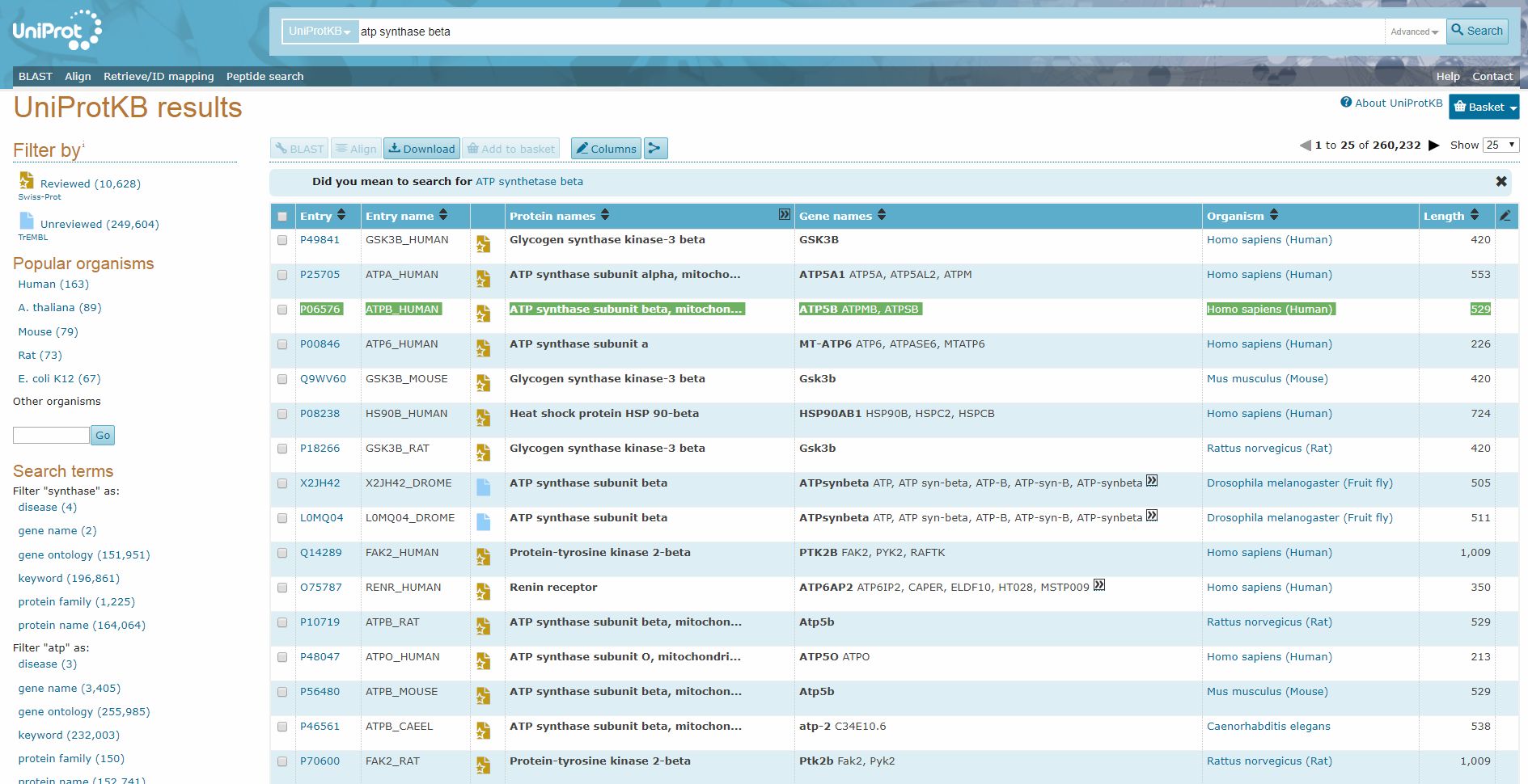
Here I searched for “ATP synthase beta”, and I found easily the human form of the beta chain:

Now, while the “Entry name”, “ATPB_human”, is a brief identifier of the protein in Uniprot, the really important ID is in the column “Entry”:  “P06576”. Indeed, this is the ID that can be used as accession number in the BLAST software, that we will discuss later.

The “Reviewed” icon in the thord column is important too, because in general it’s better to use only reviewed sequences.

By clicking on the ID in the “Entry” column, we can open the page dedicated to that protein.

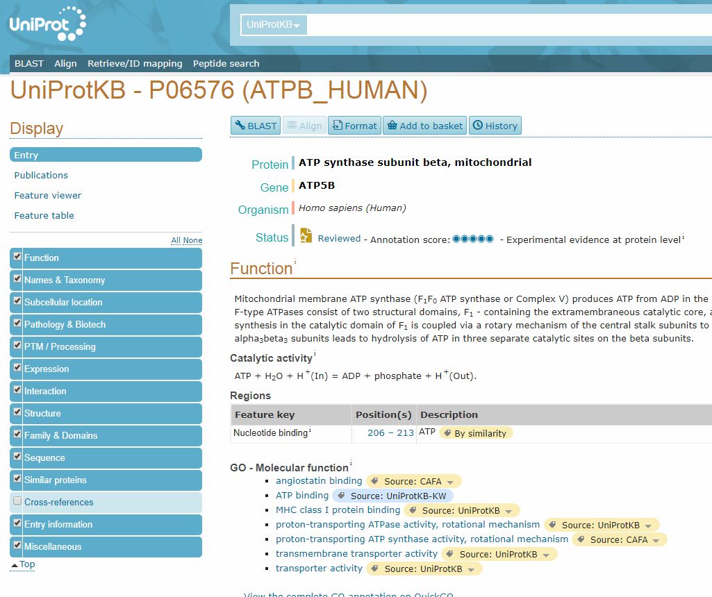
Here, we can find a lot of important information, first of all the “Function” section, which sums up what is known (or not known) about the protein function.

Another important section is the “Family and Domains” section, which gives information about domains in the protein. In this case, it just states:

Belongs to the ATPase alpha/beta chains family.

Then, the “Sequence” section gives the reference sequence for the protein:

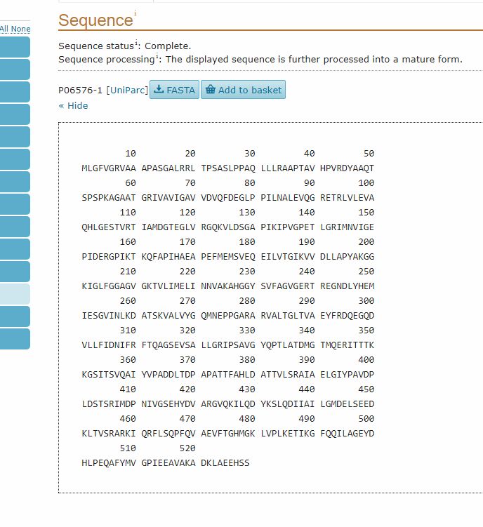
It is often useful to have the sequence in FASTA format, which is probably the most commonly used format fro sequences. To do that, we can simply click on the FASTA button (above the Sequence section). This is the result:

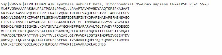
This sequence is made of two parts: a comment line, which is a summary description of the sequence, and then the sequence itself. A sequence in this form can easily be pasted into BLAST, or other bioinformatics tools, either including the comment line, or just using the mere sequence.

Now, let’s go to the second important site: BLAST (Basic Local Alignment Search Tool).  It’s a service of NCBI (National Center for Biotechnology Information).

We want to go to the Protein Blast page.

Now, let’s see how we can verify my repeated statement that the beta chain of ATP synthase is extremely conserved, from bacteria to humans. So, we past the ID from Uniprot (P06576) in the field “Accession number”, and we select Escherichia coli in the field “Organism” (important: the organism name must be selected from the drop menu, and must include the taxid number). IOWs, we are blasting the human proteins against all E. coli proteins. Here’s how it looks:

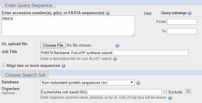
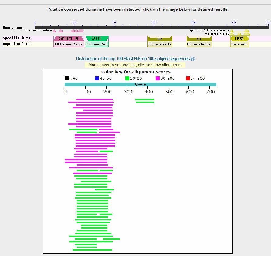
Now, we can click on the “BLAST” blue button (bottom left), and the query starts. It takes a little time. Here is the result:

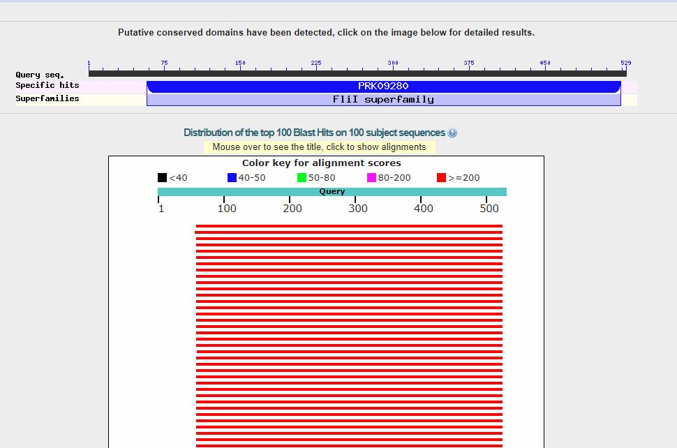
In the upper part, we can see a line representing the 529 AAs which make the protein sequence, and the recognized domains in the sequence (only one in this case).

The red lines are the hits (red, because each of them is higher than 200 bits). When you see red lines, something is there.

Going down, we see a summary of the first 100 hits, in order of decreasing homology. We can see that the first hit is with a protein named “F0F1 ATP synthase subunit beta [Escherichia coli]“, and has a bitscore of 663 bits. However, there are more than 50 hits with a bitscore above 600 bits, all of them in E. coli (that was how our query was defined), and all of them with variants of the same proteins. Such a redundancy is common, especially with bacteria, and especially with E. coli, because there are a lot of sequences available, often of practically the same protein.

Now, if we click on the first hit, or just go down, we can find the corresponding alignment:

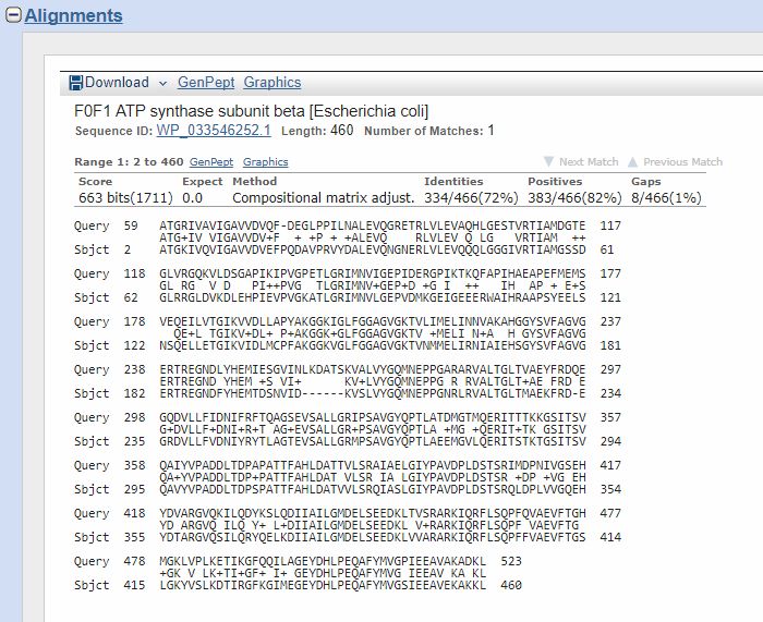
The “query” here is the human protein. You can see that the alignment involves AAs 59 – 523, corresponding tp AAs 2 – 460 of the “Subject”, that is the E. coli protein.

Th middle line represents the identities (aminoacid letter) and positives (+). The title reminds us that the hit is with a protein of E. coli whose name is “F0F1 ATP synthase subunit beta”, which is 460 AAs long (rather shorter than the human protein). It also gives us an ID/accession number for the protein, which is a different ID from Uniprot’s IDs, but can be used just the same for BLAST queries.

The important components of the result are:

1. Score: this is the bitscore, the number I use to measure functional information, provided that the homology is conserved for a long evolutionary time (usually, at least 200 – 400 million years). The bitscore is already adjusted for the properties of the scoring system.
2. The Expect number: it is simply the number of such homologies that we would expect to find for unrelated sequences (IOWs random homologies) in a similar search. This is not exactly a p value, but, as stated in the BLAST reference page: when E < 0.01, P-values and E-value are nearly identical.
3. Identities: just the number and percent of identical AAs in the two sequences, in the alignment. The percent is relative to the aligned part of the sequence, not to the total of its length.
4. Positives: the number and percent of identical + positive AAs in the alignment.  Here is a clear explanation of what “positives” are:Similarity (aka Positives)When one amino acid is mutated to a similar residue such that the physiochemical properties are preserved, a conservative substitution is said to have occurred. For example, a change from arginine to lysine maintains the +1 positive charge. This is far more likely to be acceptable since the two residues are similar in property and won’t compromise the translated protein.Thus, percent similarity of two sequences is the sum of both identical and similar matches (residues that have undergone conservative substitution). Similarity measurements are dependent on the criteria of how two amino acid residues are to each other.(From: binf.snipcademy.com)    IOWs, we could consider “positives” as “half identities”.
5. Gaps. This is the number of gaps used in the alignments. Our alignments are gapped, IOWs spaces are introduced to improve the alignment. The lower the number of gaps, the better the alignment. However, the bitscore already takes gaps in consideration, so we can usually not worry too much about them.

A very useful tool is the “Taxonomy report” (at the top of the page), which shows the hits in the various groups of organisms.

While in our example we looked only at E. coli, usually our search will include a wider range of organisms. If no organism is specified, BLAST will look for homologies in the whole protein database.

It is often useful to make queries in more groups of organisms, if necessary using the “exclude” option. For example, if I am interested in the transition to vertebrates for the SATB2 protein (ID = Q9UPW6, a protein that I have discussed in a previous OP), I can make a search in the whole metazoa group, excluding only vertebrates, as follows:

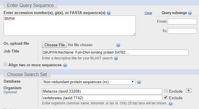
As you can see, there is very low homology before vertebrates:

And this is the taxonomy report:

The best hit is 158 bits in a spider.

Then, to see the difference in the first vertebrates, we can run a query of the same human protein on cartilaginous fish. Here is the result:

As you can see. now the best hit is 1197 bits. Quite a difference with the 158 bits best hit in pre-vertebrates.

Well, that’s what I call an information jump!

Now, my further step has been to gather the results of similar BLAST queries made for all human proteins. It is practically impossible to do that online, so I downloaded the  BLAST executables and databases. That can be done from the BLAST site, and allows one to make queries locally on one’s own computer. The use of the BLAST executables is a little more complex, because it is made by command line instructions, but it is not extremely difficult.

To perform my queries, I downloaded from Uniprot a list of all reviewed human proteins: at the time I did that, the total number was 20171. Today, it is 20239. The number varies slightly because the database is constantly modified.

So, using the local BLAST executables and the BLAST databases, I performed multiple queries of all the human proteome against different groups of organisms, as detailed in my OP here:

This kind of query take some time, from a few hours to a few days.

I have then imported the results in Excel, generating a dataset where for each  human protein (20171 rows) I have the value of protein ID, name and length, and best hit for each group of organism, including protein and organism name, protein length, bitscore value, expect value, number and percent of identities and positives, gaps. IOWs, all the results that we have when we perform a single query on the website, limited to the best hit.

In the Excel dataset I have then computed some derived variables:

• the bitscore per AA site (baa: total bitscore / human protein length)
• the information jump in bits for specific groups of organisms, in particolar between cartilaginous fish and pre-vertebrates (bitscore for cartilaginous fish – bitscore for non vertebrate deuteronomia)
• the information jump in bits per aminoacid site for specific groups of organisms, in particolar between cartilaginous fish and pre-vertebrates (baa for cartilaginous fish – baa for non vertebrate deuteronomia)

The Excel data are then imported in R. R is a wonderful open source statistical software and programming language that is constantly developed and expanded by statisticians all over the world. It also allows to create very good graphs, like the following:

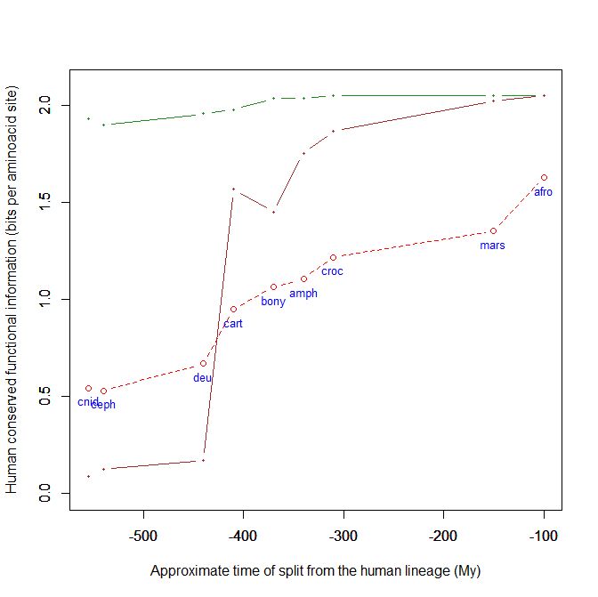
This is a kind of graph for which I have written the code and which, using the above mentioned dataset, can easily plot the evolutionary history, from cnidaria to mammals, of any human protein, or group of protein, using their IDs. This graph uses the bit per aminoacid values, and therefore sequences of different length can easily be compared. A refernce line is always plotted, with the mean baa value in each group of organism for all human proteins. That already allows to visualize how the pre-vertebrate-vertebrate transition exhibitis the greatest informational jump, in terms of human conserved information.

However, the plots regarding individual proteins are much more interesting, and they reveal huge differences in the their individual histories. In the above graph, for example, I have plotted the histories of two completely different proteins:

1. The green line is protein Cdc42, “a small GTPase of the Rho family, which regulates signaling pathways that control diverse cellular functions including cell morphology, cell migration, endocytosis and cell cycle progression” (Wikipedia). It is 191 AAs long, and, as can be seen in the graph, it is extremely conserved in all metazoa, presented almost maximal homology with the human form already in Cnidaria.
2. The brown line is our well known SATB2 (see above), a 733 AAs protein which is, among other things, “required for the initiation of the upper-layer neurons (UL1) specific genetic program and for the inactivation of deep-layer neurons (DL) and UL2 specific genes, probably by modulating BCL11B expression. Repressor of Ctip2 and regulatory determinant of corticocortical connections in the developing cerebral cortex.” (Uniprot) In the graph we can admire its really astounding information jump in vertebrates.

This kind of graph is very good to visualize the behaviour of proteins and of groups of proteins. For example, the following graph is of proteins involved in neuronal adhesion:

It shows, as expected, a big information jump, mainly in cartilaginous fish.

The following, instead, is of odorant receptors:

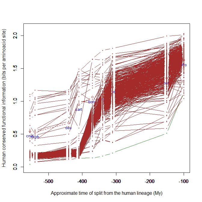
Here, for example, the jump is later, in bony fish, and it goes on in amphibian and reptiles, and up to mammals.

Well, I think that I have given at least a general idea of the main issues and procedures. If anyone has specific requests, I am ready to answer.